NUCLEAR PHYSICS AND INTERDISCIPLINARY RESEARCH
Reducing systematic bias in machine learning applications to J/ψ signal extraction in high-energy nuclear physics
Nuclear Science and Techniques|Vol. 37, No. 8|Article ID: 145|Print 2026-08|Online 2026-05-20
DOI: 10.1007/s41365-026-01985-4CSTR: 32136.14.NST.2026.08145
Machine-learning techniques are increasingly used in high-energy nuclear physics because they can exploit multivariate correlations more efficiently than conventional cut-based analyses. A central challenge is the construction of training samples that faithfully reproduce the detector response observed in data. Signal samples are usually derived from detector simulations; therefore, mismatches between simulation and data can degrade classifier performance and introduce systematic biases. This work presents two practical correction procedures, namely cumulative distribution function (CDF) mapping and a shift-and-scale transformation, to align simulated signal features with those measured in data. Their performance is demonstrated with J/ψ yield measurements in sNN=200 GeV Ru+Ru and Zr+Zr collisions recorded by STAR. A set of self-consistency tests shows that these procedures substantially suppress the systematic bias associated with data-simulation discrepancies in machine-learning-based signal extraction.
Introduction
Machine learning has become an indispensable tool across a broad range of scientific and technological disciplines, including image recognition, natural-language processing, recommendation systems, and speech analysis. Its main advantage is the ability to identify complex structures in high-dimensional datasets and to provide powerful tools for classification, regression, and clustering [1-6]. In nuclear physics, machine learning has been used to extract or predict key observables such as charge radii, nuclear masses, and binding energies [7-11]. In relativistic heavy-ion collisions, it is especially valuable for classification tasks, for example separating rare physics signals from large combinatorial backgrounds [12-17]. Representative algorithms include boosted decision trees (BDTs) [18, 19], deep neural networks [20-22], and ensemble methods [23], all of which can exploit multidimensional correlations more effectively than conventional straight-cut analyses. Independent of the specific algorithm, a reliable classifier requires representative signal and background samples. Whereas background samples can often be obtained directly from data, signal samples are usually produced with Monte Carlo simulations. Because detector simulations do not perfectly reproduce the data, training on mismatched signal samples can degrade classifier performance and bias the extracted physics observables, as illustrated in Appendix 7.
To address this challenge, we propose two correction methods: cumulative distribution function (CDF) mapping and shift-and-scale. CDF mapping systematically transforms a simulated feature distribution into the corresponding distribution measured in data without requiring an explicit parametric description of the shape, which makes it flexible and broadly applicable. The shift-and-scale procedure is more restrictive but simpler to implement, and it is well suited to cases in which the simulated and measured distributions already have similar shapes and differ mainly in location and width.
J/ψ is a classic probe of the medium created in relativistic heavy-ion collisions and is widely used to investigate the properties of the Quark–Gluon Plasma [24, 25]. Accurate yield measurements are therefore of continuing interest [26-34]. In this work, a BDT implemented with the eXtreme Gradient Boosting (XGBoost) framework [35] is used to separate the J/ψ signal from background in Ru+Ru and Zr+Zr collisions at  GeV recorded by STAR at RHIC. This case study demonstrates both the implementation of the proposed correction procedures and their effectiveness in improving the robustness of machine-learning-based signal extraction. Section 2 describes the J/ψ reconstruction, Sections 3 and 4 present the construction of the training samples and the model training procedure, Sect. 5 discusses the self-consistency tests and results, and Sect. 6 summarizes the main conclusions.
J/ψ Reconstruction
In 200 GeV Ru+Ru and Zr+Zr collisions, J/ψ mesons are reconstructed through the dielectron decay channel [27, 34, 36], with electron1 identification based on the Time-of-Flight (TOF) [37], the Time Projection Chamber (TPC) [38, 39], and the Barrel Electromagnetic Calorimeter (BEMC) [40] detectors. Loose preselection requirements on the particle-identification (PID) observables are first imposed to suppress the dominant background while retaining sufficient signal statistics for the subsequent machine-learning analysis.
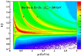
The TOF detector measures the arrival time of a charged particle. Together with the collision start time and the momentum measured in the TPC, one obtains  , where c is the speed of light and v is the particle velocity. Figure 1 shows the distribution of 1/β as a function of momentum p for charged particles. Because particles with different masses have different velocities at the same momentum, distinct PID bands appear in this representation. A preselection cut of
 is applied, shown as dashed lines in Fig. 1 and listed in Table 1.
Electron preselection cuts and the optimal BDT cut criterion from machine learning

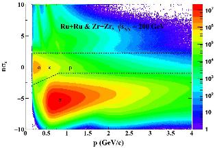
The TPC measures the specific ionization energy loss, dE/dx, which provides additional separation between electrons and hadrons. PID based on dE/dx is commonly expressed through the normalized deviation of the measured value from the expectation for a given particle species, denoted by nσe, nσπ, and so forth. For electrons, the nσe distribution is expected to be approximately Gaussian with mean 0 and width 1 after proper calibration. Figure 2 shows the nσe distribution as a function of p after imposing a tighter TOF requirement,  , to improve the electron purity for visualization. The dashed curves indicate the momentum-dependent preselection criteria used before machine-learning training.
 cut. The dashed curves correspond to the nσe cuts used for electron preselection
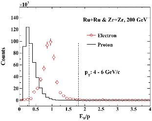
At high momentum, the BEMC provides additional PID through the ratio of the deposited electromagnetic energy to the track momentum. In practice, electron identification commonly uses the largest tower energy within the BEMC cluster, E0, rather than the total cluster energy Etot, because E0 has better resolution and is less sensitive to the high detector occupancy in heavy-ion collisions. Figure 3 compares the E0/p distributions for protons and electrons in the range 4<pT<6 GeV/c. The electron sample, often referred to as photonic electrons, is obtained from photon conversions and neutral-meson Dalitz decays [41]. As expected, the electron distribution peaks at a larger E0/p value than the proton distribution. The dashed vertical lines indicate the preselection requirement on E0/p.
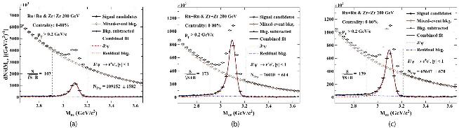
The use of the TOF, TPC, and BEMC preselection criteria depends on the track kinematics and on whether matching information is available in the TOF and BEMC, as summarized in Table 1. Electron and positron candidates that satisfy these requirements are paired to form J/ψ candidates, and the resulting invariant-mass distribution is shown in Fig. 4(a). The combinatorial background is estimated with the mixed-event technique [42]. After subtracting this component, the remaining invariant-mass distribution is fitted with two terms: a Crystal Ball function for the J/ψ signal and a linear term for the residual background arising mainly from semileptonic heavy-flavor decays and Drell–Yan production. The raw J/ψ yield is obtained by counting the electron–positron pairs in the mass window [2.91, 3.21] GeV/c2 and subtracting the fitted residual-background contribution in the same interval. Approximately  J/ψ candidates are reconstructed, with a signal significance of 103. The following sections show how machine learning further improves this significance.
 and pT > 0.2 GeV/c, for Ru+Ru and Zr+Zr collisions. Different panels correspond to different electron identification cuts. (a) With preselection cuts listed in Table 1; (b) With preselection and BDT cuts listed in Table 1; (c)With straight cuts listed in Table 2
Construction of Training Samples
For J/ψ reconstruction, the classification targets are electron–positron pairs that form J/ψ candidates. To determine whether a candidate is signal-like or background-like, a set of discriminating features must be defined. In principle, any observable that improves the separation without introducing physics bias can be used. In this work, the selected features are nσe, nσπ, E0/p, and the distance of closest approach (DCA, defined as the minimum distance between a charged-particle trajectory and the collision vertex) for both daughter tracks, labeled as “tr1” and “tr2”.
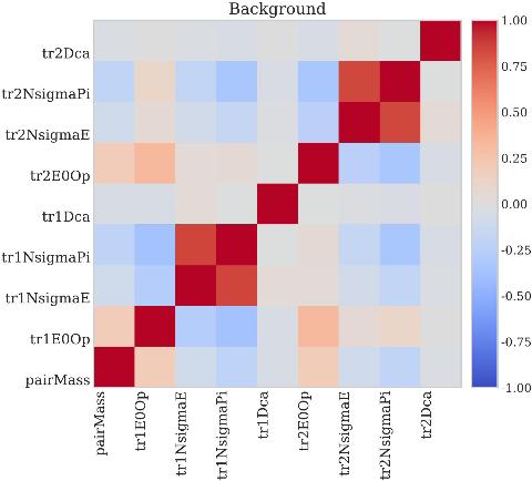
The background training sample is selected from electron–positron pairs in the invariant-mass sidebands, namely (2.65, 2.85), (3.25, 3.5), and (3.8, 4.5) GeV/c2, well separated from the J/ψ peak. The interval (3.5, 3.8) GeV/c2 is excluded because it contains a small contribution from  mesons. This sideband method assumes that the background in the sidebands is representative of the background beneath the J/ψ peak. Therefore, the features used for classification should not depend strongly on the pair invariant mass, which constitutes an important feature-selection criterion. Figure 5 shows the correlations between the selected features and the invariant mass for the background sample; no strong mass dependence is observed. As expected, nσe and nσπ are strongly correlated because both are derived from the same dE/dx measurement.
The signal training sample is generated with Monte Carlo simulation. Electrons and positrons from J/ψ decays are propagated through a GEANT3-based [43] model of the STAR detector, and the simulated hits are embedded into real Ru+Ru and Zr+Zr events before reconstruction with the same software chain used for data. Inevitably, the simulation does not perfectly reproduce the data because detector conditions evolve with time and the heavy-ion environment has high occupancy. The quality of the simulation can be assessed by comparing the nσe, nσπ, E0/p, and DCA distributions for electrons from simulated J/ψ decays with those for photonic electrons in data, as shown in Fig. 6. The DCA distributions agree reasonably well, whereas the nσe and nσπ distributions exhibit clear offsets and the E0/p distribution shows a noticeable shape mismatch. If left uncorrected, these discrepancies can degrade the machine-learning performance and bias the extracted J/ψ yield.
 GeV/c and
 from simulations, both with (open diamonds) and without (filled diamonds) corrections, to those from real data (filled circles). (a) nσe distributions; (b) nσπ distributions; (c) E0/p distributions; (d) DCA distributions
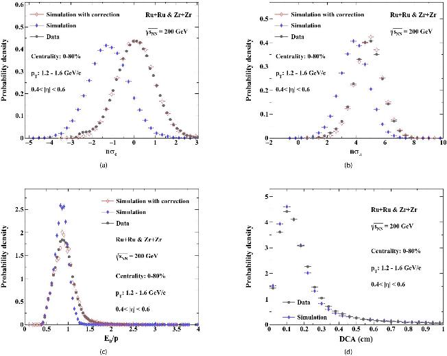
Because the simulated and measured nσe and nσπ distributions have similar shapes, they can be corrected with a shift-and-scale transformation: (1)Here, μdata (σdata) and μsimu (σsimu) are the means (standard deviations) of the corresponding nσi distributions in data and simulation, respectively, with i=e or π. After this transformation, the simulated nσe and nσπ distributions agree well with those observed in data, as shown in Fig. 6(a) and (b).
For the E0/p distribution, the mismatch between simulation and data is not limited to a simple offset or width difference, so shift-and-scale is insufficient. We therefore introduce a cumulative distribution function (CDF) mapping method. Let  and
 , with
 , denote the probability density functions of a feature in simulation and data, respectively. The corresponding CDF is
 DF2For an event in simulation with feature value A, its cumulative probability is
 DF3The corrected value B is then obtained from the data distribution through
 DF4This procedure defines an event-by-event mapping from the original value A to the corrected value B, such that the transformed simulation reproduces the data distribution. After CDF mapping, the corrected simulated E0/p distribution (open diamonds) is consistent with the distribution measured in data (solid circles), as shown in Fig. 6(c). In practice, the PDFs are represented by discrete histograms, so the method is implemented numerically by constructing discrete CDFs and searching for the closest cumulative probability. When the simulation and data differ strongly in shape, this discrete matching can produce bin-to-bin fluctuations at the level of one histogram bin, leading to localized excesses in some bins and deficits in neighboring bins. This effect explains the statistical irregularities visible in Fig. 6(c). Because the classifier is trained on event-by-event continuous feature values rather than on the displayed histogram counts themselves, this binning artifact does not compromise the model training. It can be further reduced by decreasing the histogram bin width.
Compared with shift-and-scale, CDF mapping is more general but also more involved to implement. Both procedures act deterministically on each event and therefore retain the event-level correspondence among observables, which is essential for multivariate classifiers to benefit from joint feature information. For the same reason, the signal sample cannot be constructed by independently sampling one-dimensional feature distributions from data, because that procedure would destroy the physically relevant inter-feature dependence structure.
Model Training and Application
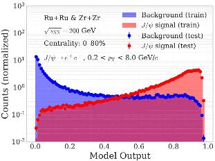
A BDT classifier implemented with XGBoost is trained to further improve the J/ψ signal significance. The signal and background samples are each divided into two equal subsets, one for training and the other for testing. After training, the model is applied to both subsets. For every electron–positron pair, the classifier returns an output between 0 and 1, with values close to 1 corresponding to signal-like candidates and values close to 0 corresponding to background-like candidates. The output distributions are shown in Fig. 7. The red band and red points denote the signal distributions for the training and testing samples, respectively, whereas the blue band and blue points show the corresponding background distributions. The strong separation between signal and background indicates good discriminating power, and the agreement between the training and testing samples shows that overtraining is not evident.
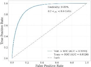
In the final analysis, a threshold on the BDT output is chosen so that pairs with scores above the threshold are retained as signal candidates and those below it are rejected as background. For a given threshold, the signal efficiency is defined as the fraction of signal events that survive the cut, and the background efficiency is defined analogously. Plotting the signal efficiency against the background efficiency while scanning the threshold from 0 to 1 yields the receiver operating characteristic (ROC) curve, where the horizontal and vertical axes correspond to the false-positive rate (FPR) and true-positive rate (TPR), respectively. The ROC curves for the training and testing samples are shown in Fig. 8. The area under the curve (AUC) quantifies the overall classification performance; values closer to 1 indicate better separation. The AUC obtained here is 0.91, demonstrating strong discriminating power. The nearly identical ROC curves and AUC values for the training and testing samples provide additional evidence that the model is not overfit.
Model Validation via Self-Consistency Checks
Beyond establishing that the model is not overtrained, it is necessary to verify that the BDT efficiencies for both signal and background are correctly reproduced in real data. This validation is carried out through two self-consistency tests.
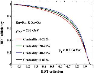
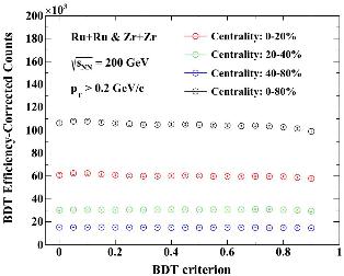
The first test examines the J/ψ yield corrected for the BDT efficiency as a function of the BDT threshold. Because the measured yield should not depend on the particular analysis threshold, the corrected yield is expected to remain constant within uncertainties. The J/ψ efficiency for a given BDT threshold is derived from the signal output distribution in Fig. 7, and the resulting efficiency curves are shown in Fig. 9 for several centrality intervals in Ru+Ru and Zr+Zr collisions. Here, centrality characterizes the geometric overlap of the two nuclei: 0–20% corresponds to the most central collisions, whereas 40–80% corresponds to more peripheral collisions. After applying the preselection criteria in Table 1 and varying the BDT threshold, the raw J/ψ counts are extracted from data with the procedure described in Sect. 2. Figure 10 then shows the efficiency-corrected J/ψ counts as a function of the BDT threshold for four centrality classes. Although the signal efficiency changes by roughly an order of magnitude as the threshold increases from 0 to 0.9, the corrected counts remain stable, with variations below 2%. This stability strongly suggests that the signal-efficiency estimate from the machine-learning model accurately represents the efficiency in data, thereby validating the feature-correction procedure described in Sect. 3.
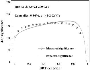
A more stringent validation compares the J/ψ significance as a function of the BDT threshold between the machine-learning expectation and the measurement in data, because this test depends on both the signal and background efficiencies. The expected J/ψ significance is calculated as (2)In Eq. 2, x is the BDT threshold, and
 and
 are the corresponding signal and background efficiencies. The quantities S(x) and B(x) denote the signal and background counts after the threshold is applied, while S0 and B0 are the counts at a reference threshold x0. The choice of x0 is arbitrary and is used only to normalize the prediction to the data at one point. The resulting expected significance is shown as the gray band in Fig. 11. It first increases and then decreases as the threshold is tightened from 0 to 0.9, reflecting the competition between improved background rejection and reduced signal efficiency. The prediction from the trained model is compared with the significance extracted directly from data, shown as open circles. For clarity, the two curves are aligned at a threshold of 0.5, namely x0=0.5 in Eq. 2. Their consistency indicates that the training samples reproduce the behavior of both signal and background in data with sufficient accuracy for this analysis.
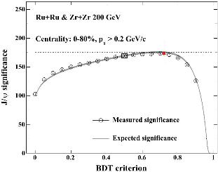
The expected-significance curve from the trained model also provides a principled way to determine the optimal BDT threshold. Compared with scanning the data directly, an optimization based on the training samples is less sensitive to statistical fluctuations in the measured spectrum and therefore less prone to introducing threshold-selection bias, which is particularly important for low-statistics signals. As shown in Fig. 11, the J/ψ significance reaches its maximum at a BDT threshold of 0.72, which is therefore chosen as the working point. Figure 4(b) shows the raw signal extraction obtained with this optimal threshold. The corresponding significance is 173, representing a 68% improvement over the result with only the preselection criteria [Fig. 4(a)] and a 24% improvement over the result obtained with straight PID cuts [Fig. 4(c) and Tab. 2].
Straight cuts used for electron identification

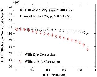
The same self-consistency tests are also useful for diagnosing problematic input features. If adding a given feature destroys the agreement between the model expectation and the data, that feature should be corrected or removed from the training. As an example, Fig. 12 in the Appendix shows the result obtained without CDF mapping for E0/p. In that case, the efficiency-corrected signal counts deviate progressively from the expected flat behavior as the BDT threshold increases, reaching 29% at a threshold of 0.9. Likewise, the expected J/ψ significance becomes inconsistent with the significance measured in data, as shown in Fig. 13. These discrepancies provide direct evidence that the feature-correction procedures introduced in Sect. 3 are necessary for unbiased signal extraction.
Summary
This work develops two practical procedures, CDF mapping and shift-and-scale, to align simulated feature distributions with those measured in data while preserving the event-level multivariate information required for machine-learning classification. These methods address a common source of systematic bias in experimental analyses, namely the mismatch between simulated and real detector responses. Using J/ψ yield extraction in  GeV Ru+Ru and Zr+Zr collisions as a case study, we show that the corrected training samples lead to stable efficiency-corrected yields and to a predicted significance consistent with the significance measured in data. The self-consistency tests therefore validate both the necessity and the effectiveness of the proposed corrections. The same strategy should be broadly useful in machine-learning applications throughout high-energy nuclear and particle physics whenever simulated signal samples do not fully reproduce the data.
References
1..
LeCun Y., Bengio Y., Hinton G., Deep learning. Nature 521, 436–444 (2015). https://doi.org/10.1038/nature14539
2..
PANG L., Zhou K., Wang X., Deep Learning for Nuclear Physics. Nucl. Phys. Rev. 37(3), 720–726 (2020). https://doi.org/10.11804/NuclPhysRev.37.2019CNPC41
3..
Li F.P., Pang L.G., Qin G.Y., QCD equation of state at finite μB using a deep learning-assisted quasi-parton model. Phys. Lett. B 868, 139692 (2025). https://doi.org/10.1016/j.physletb.2025.139692
4..
He W., Li Q., Ma Y. et al., Machine learning in nuclear physics at low and intermediate energies. Sci. China Phys. Mech. Astron. 66(8), 282001 (2023). https://doi.org/10.1007/s11433-023-2116-0
5..
Li Z., Wang Y., Li Q. et al., Machine-learning predictions for the nuclear charge radius: Bayesian method versus decision-tree-based algorithm. Phys. Rev. C 112(1), 014312 (2025). https://doi.org/10.1103/vj25-zwd3
6..
Niu Z.M., Fang J.Y., Niu Y.F., Comparative study of radial basis function and Bayesian neural network approaches in nuclear mass predictions. Phys. Rev. C 100(5), 054311 (2019). https://doi.org/10.1103/PhysRevC.100.054311
7..
Zhou B., Cao Y.Y., Guo J.Y., Predictions of nuclear charge radii based on the convolutional neural network. Nucl. Sci. Tech. 34(10), 152 (2023). https://doi.org/10.1007/s41365-023-01308-x
8..
Li Q.F., Wang Y.J., Gao Z.P. et al., Machine learning the nuclear mass. Nucl. Sci. Tech. 32(10), 109 (2021). https://doi.org/10.1007/s41365-021-00956-1
9..
Tang L., Zhang Z.H., Nuclear charge radius predictions by kernel ridge regression with odd-even effects. Nucl. Sci. Tech. 35(2), 19 (2024). https://doi.org/10.1007/s41365-024-01379-4
10..
Ren Z.Z., Yuan Z.Y., Bai D. et al., Reliable calculations of nuclear binding energies by the gaussian process of machine learning. Nucl. Sci. Tech. 35(6), 105 (2024). https://doi.org/10.1007/s41365-024-01463-9
11..
Zhang G.Q., Cao X.G., Cheng G.Y. et al., The study of intelligent algorithm in particle identification of heavy-ion collisions at low and intermediate energies. Nucl. Sci. Tech. 35(2), 33 (2024). https://doi.org/10.1007/s41365-024-01388-3
12..
Albertsson K., Altoe P., Anderson D. et al., Machine Learning in High Energy Physics Community White Paper. J. Phys. Conf. Ser. 1085(2), 022008 (2018). https://doi.org/10.1088/1742-6596/1085/2/022008
13..
Sirunyan A.M., Tumasyan A., Adam A. et al. (CMS), Identification of heavy, energetic, hadronically decaying particles using machine-learning techniques. JINST 15(06), P06005 (2020). https://doi.org/10.1088/1748-0221/15/06/P06005
14..
Acharya S., Adamová D., Agarwal A. et al. (ALICE), Measurement of beauty production via non-prompt charm hadrons in p–Pb collisions at sNN=5.02 TeV. JHEP 11, 148 (2024). https://doi.org/10.1007/JHEP11(2024)148
15..
Acharya S.,Adamová D., Adler A. et al. (ALICE), First measurement of Ωc0 production in pp collisions at s=13 TeV. Phys. Lett. B 846, 137625 (2023). https://doi.org/10.1016/j.physletb.2022.137625
16..
Acharya S.,Adamová D., Adler A. et al. (ALICE), First measurement of Λc+ production down to pT=0 in pp and p–Pb collisions at sNN=5.02 TeV. Phys. Rev. C 107(6), 064901 (2023). https://doi.org/10.1103/PhysRevC.107.064901
17..
Acharya S.,Adamová D., Aglieri Rinella G. et al. (ALICE), Study of flavor dependence of the baryon-to-meson ratio in proton-proton collisions at s=13 TeV. Phys. Rev. D 108(11), 112003 (2023). https://doi.org/10.1103/PhysRevD.108.112003
18..
Coadou Y., Boosted decision trees. in Artificial Intelligence for High Energy Physics, ed. by Calafiura P., Rousseau D., Terao K. (World Scientific, Singapore, 2022), pp. 9–58. https://doi.org/10.1142/9789811234033_0002
19..
Roe B.P., Yang H.J., Zhu J., Liu Y. et al., Boosted decision trees, an alternative to artificial neural networks. Nucl. Instrum. Meth. A 543(2-3), 577–584 (2005). https://doi.org/10.1016/j.nima.2004.12.018
20..
Schmidhuber J., Deep learning in neural networks: An overview. Neural Networks 61, 85–117 (2015). https://doi.org/10.1016/j.neunet.2014.09.003
21..
Madrazo C.F., Cacha I.H., Iglesias L.L., de Lucas J.M., Application of a Convolutional Neural Network for image classification for the analysis of collisions in High Energy Physics. EPJ Web Conf. 214, 06017 (2019). https://doi.org/10.1051/epjconf/201921406017
22..
Baldi P., Bauer K., Eng C. et al., Jet Substructure Classification in High-Energy Physics with Deep Neural Networks. Phys. Rev. D 93(9), 094034 (2016). https://doi.org/10.1103/PhysRevD.93.094034
23..
Bentley I., Tedder J., Gebran M. et al., High precision binding energies from physics-informed machine learning. Phys. Rev. C 111(3), 034305 (2025). https://doi.org/10.1103/PhysRevC.111.034305
24..
Matsui T., Satz H., J/ψ Suppression by Quark-Gluon Plasma Formation. Phys. Lett. B 178, 416–422 (1986). https://doi.org/10.1016/0370-2693(86)91404-8
25..
The QGP discovered at RHIC. In: Greiner W., Itkis M.G., Reinhardt J., Güçlü M.C. (eds) Structure and dynamics of elementary matter. NATO Science Series (Springer, Dordrecht, 2004). vol 166, pp. 159–182. https://doi.org/10.1007/978-1-4020-2705-5_1426.L.Adamczyk
26..
Adamczyk L. et al. (STAR), J/ψ production at low pT in Au + Au and Cu + Cu collisions at sNN=200 GeV with the STAR detector. Phys. Rev. C 90(2), 024906 (2014). https://doi.org/10.1103/PhysRevC.90.024906
27..
Adamczyk L., Agakishiev G., Aggarwal M.M. et al. (STAR), J/ψ production at high transverse momenta in p+p and Au+Au collisions at sNN=200 GeV. Phys. Lett. B 722, 55–62 (2013). https://doi.org/10.1016/j.physletb.2013.04.010
28..
Adamczyk L., Adkins J.K., Agakishiev G. et al. (STAR), Energy dependence of J/ψ production in Au+Au collisions at sNN=39, 62.4 and 200 GeV. Phys. Lett. B 771, 13–20 (2017). https://doi.org/10.1016/j.physletb.2017.04.078
29..
Adare A.,Afanasiev S., Aidala C. et al. (PHENIX), J/ψ Production vs Centrality, Transverse Momentum, and Rapidity in Au+Au Collisions at sNN=200 GeV. Phys. Rev. Lett. 98, 232301 (2007). https://doi.org/10.1103/PhysRevLett.98.232301
30..
Abelev B.B.,Adam J., Adamová D. et al. (ALICE), Centrality, rapidity and transverse momentum dependence of J/ψ suppression in Pb-Pb collisions at sNN=2.76 TeV. Phys. Lett. B 734, 314–327 (2014). https://doi.org/10.1016/j.physletb.2014.05.064
31..
Adam J.,Adamová D., Aggarwal M.M. et al. (ALICE), Inclusive, prompt and non-prompt J/ψ production at mid-rapidity in Pb-Pb collisions at sNN=2.76 TeV. JHEP 07, 051 (2015). https://doi.org/10.1007/JHEP07(2015)051
32..
Adam J.,Adamczyk L., Adams J.R. et al. (STAR), Measurement of inclusive J/ψ suppression in Au+Au collisions at sNN=200 GeV through the dimuon channel at STAR. Phys. Lett. B 797, 134917 (2019). https://doi.org/10.1016/j.physletb.2019.134917
33..
Wang Y. (STAR), J/ψ production in Ru+Ru and Zr+Zr collisions at sNN=200 GeV with the STAR experiment. PoS HardProbes2023, 110 (2024). https://doi.org/10.22323/1.438.0110
34..
Tang Z., Zha W., Zhang Y., An experimental review of open heavy flavor and quarkonium production at RHIC. Nucl. Sci. Tech. 31(8), 81 (2020). https://doi.org/10.1007/s41365-020-00785-8
35..
Chen T., Guestrin C., XGBoost: A Scalable Tree Boosting System (2016). https://doi.org/10.1145/2939672.2939785
36..
Chen J.,Dong X., He X.H. et al., Properties of the QCD matter: review of selected results from the relativistic heavy ion collider beam energy scan (RHIC BES) program. Nucl. Sci. Tech. 35(12), 214 (2024). https://doi.org/10.1007/s41365-024-01591-2
37..
Llope W.J. (STAR), The large-area time-of-flight (TOF) upgrade for the STAR detector. AIP Conf. Proc. 1099(1), 778–781 (2009). https://doi.org/10.1063/1.3120153
38..
Wieman H.,Anderssen E., Banerjee A. et al. (STAR), STAR TPC at RHIC. IEEE Trans. Nucl. Sci. 44, 671–678 (1997). https://doi.org/10.1109/23.603731
39..
Anderson M.,Berkovitz J., Betts W. et al., The Star time projection chamber: A Unique tool for studying high multiplicity events at RHIC. Nucl. Instrum. Meth. A 499, 659–678 (2003). https://doi.org/10.1016/S0168-9002(02)01964-2
40..
Beddo M.,Bielick E., Fornek T. et al. (STAR), The STAR barrel electromagnetic calorimeter. Nucl. Instrum. Meth. A 499, 725–739 (2003). https://doi.org/10.1016/S0168-9002(02)01970-8
41..
Adamczyk L.,Adkins J.K., Agakishiev G. et al. (STAR), Measurements of Dielectron Production in Au+Au Collisions at sNN=200 GeV from the STAR Experiment. Phys. Rev. C 92(2), 024912 (2015). https://doi.org/10.1103/PhysRevC.92.024912
42..
Adare A.,Afanasiev S., Aidala C. et al. (PHENIX), Detailed measurement of the e+e- pair continuum in p+p and Au+Au collisions at sNN=200 GeV and implications for direct photon production. Phys. Rev. C 81, 034911 (2010). https://doi.org/10.1103/PhysRevC.81.034911
43..
Abelev B.I.,Aggarwal M.M., Ahammed Z. et al. (STAR), Systematic Measurements of Identified Particle Spectra in pp, d+Au and Au+Au Collisions from STAR. Phys. Rev. C 79, 034909 (2009). https://doi.org/10.1103/PhysRevC.79.034909